Simulation: a toolset for virtual experiments

2. CAD-Integrated Simulation Tools: Fusion 360, Solidworks

2.2 Tutorial #1: Static Stress Simulation of a Rod Assembly

2.3 Tutorial #2: Shape Optimization of Robotic Arm Gripper

3. Advanced Multiphysics Simulation Tools: Simulia - Comsol

3.2 Tutorial #3:Capacitive Sensing

4. Object-Oriented Modeling & Simulation: Open Modelica, Matlab-Simulink

5. Custom Design Tools with Simulation Capabilities

1. Basic Concepts

1.1 System-Model-Experiments

In HTMAA we built systems. We usually start from CAD models and we end to physical models using rapid prototyping techniques. Sometimes the systems we want to build haven't been realized before and we would like to know if we violate physics before we start our fab adventure...Sometimes these systems have already been realized but we want to design new ones with better performance...
The purpose of this recitation is to see the tools that we have in our availability in order to test our system ideas in a computer environment by performing virtual experiments.

1.2 Mathematical Model

A mathematical model is a description of a system where the relationships between variables of the system are expressed in mathematical form. Variables can be measurable quantities such as size, length, weight, temperature, unemployment level, information flow, bit rate, and so forth. Most laws of nature are mathematical models in this sense. For example, Ohm’s law describes the relationship between current and voltage for a resistor; Newton’s laws describe relationships between velocity, acceleration, mass, force

Mathematical models usually contain equations. There are basically four main kinds of equations:
- Differential equations contain time derivatives such as dx/dt
- Algebraic equations do not include any differentiated variables
- Partial differential equations also contain derivatives with respect to both space and time.
- Difference equations express relations between variables, for example, at different points in time.
Types of Mathematical Models:
- Dynamic vs Static Models - Continuous-Time vs Discrete-Time

1.3 Simulation

Definition:
In our case, a simulation is an experiment performed on a CAD model, whereby a numerical technique (finite elements) is used to solve the equations that describe the physics of the system.

Why simulations?
- Experiments are too expensive, too dangerous, or the system to be investigated does not yet exist.
- The time scale of the dynamics of the system is not compatible with that of the experimenter. For example, it takes millions of years to observe small changes in the development of the universe, whereas similar changes can be quickly observed in a computer simulation of the universe.
- Variables may be inaccessible. In a simulation all variables can be studied and controlled, even those that are inaccessible in the real system.
- Easy manipulation of models. Using simulation, it is easy to manipulate the parameters of a system model, even outside the feasible range of a particular physical system. For example, the mass of a body in a computer-based simulation model can be increased from 40 to 500 kg at a keystroke, whereas this change might be hard to realize in the physical system.
- Suppression of disturbances. In a simulation of a model it is possible to suppress disturbances that might be unavoidable in measurements of the real system. This can allow us to isolate particular effects and thereby gain a better understanding of those effects.
- Suppression of second-order effects. Often, simulations are performed since they allow suppression of second-order effects such as small non-linearities or other details of certain system components, which can help us to better understand the primary effects.

Dangers of simulation!
- Falling in love with a model—the Pygmalion1 effect. It is easy to become too enthusiastic about a model and forget all about the experimental frame, that is, that the model is not the real world but only represents the real system under certain conditions.
- Forcing reality into the constraints of a model—the Procrustes effect.
- Forgetting the model’s level of accuracy. All models have simplifying assumptions, and we have to be aware of those in order to correctly interpret the results.

2. CAD-Integrated Simulation Tools: Solidworks, Fusion 360

2.1 Overview

Solidworks:
- Simulation Capabilities
- Force Spring Animation
- Flow Animation
- Injection Molding Animation
- Fluid Structure Interaction
- Awesome Highlight Animations

Fusion 360:
- Simulation Capabilities
- FEA Mesh Basics

2.2 Tutorial #1: Static Stress Simulation of a Rod Assembly

In this video, we talk about Static Stress analyses—specifically, their purpose, workflow, capabilities, and what results they produce. Perform a static stress analysis to determine stress, strain, displacement, and safety factor, in a part or assembly resulting from various applied loads. You can also determine contact pressures between parts of an assembly. In order for this type of study to be valid, the model must have the following characteristics.
- For accurate results, stresses cannot exceed the yield strength of the materials.
- The loading must cause only small deflections or rotations. So, deformation can’t have a significant effect on the load direction, magnitude, or the surface area to which loads are applied. Also, the deformation can’t alter where, or in what manner, the parts are constrained.
- Finally, dynamic effects from the loading are not significant. Static stress analyses do not consider damping or inertial effects (that is, momentum).
This model is a three-part assembly consisting of a connecting rod and two round pins. A 2,000-pound tensile load is applied to the assembly. Separation contact is defined between the parts, meaning that the pins can freely slide along or separate from the connecting rod. But the parts can’t penetrate through each other.
Let’s take a look at the process of setting up and solving the analysis.
The first time you enter the SIMULATION workspace, the New Study dialog launches automatically. Choose the Static Stress analysis type. Click this icon to access the study settings. We’ll define an absolute mesh size of 0.125 inch, which will produce two elements through the thickness in the thinnest regions of the connecting rod.
If you want to make changes to the model for your simulation, use the Simplify command. The tools in the SIMPLIFY workspace enable you to: remove unnecessary components or features; split faces to confine a load or constraint to only a portion of a larger face, or to provide edges or vertices for locating loads and constraints; or modify the geometry in any way you want to achieve the desired results. Any changes you make here affect only the simulation model. The production geometry represented in the MODEL workspace remains unchanged. Click Finish Simplify to return to the SIMULATION workspace.
The materials were previously defined in the MODEL workspace. We’ll confirm that the study materials match the model materials. Let’s apply the following constraints to make the model statically stable without impeding its expected displacement under load:
- Fully fix the ends of the small pin.
- Apply a Z constraint to the straight edges on the large pin. This constraint prevents the pin from spinning in its hole and prevents the connecting rod from rotating about the centerline of the small pin.
- Apply a Y constraint to the pin and connecting rod edges at the middle of the large hole. This constraint prevents the connecting rod from sliding axially along the small pin, and it prevents the large pin from sliding axially in the large hole.
Next, apply a total load of 2,000 pounds in the -X direction to the ends of the large pin. Automatically detect all contact sets. The default tolerance is fine because the parts are touching at each contact face. Edit all contact sets to change the Contact Type from Bonded to Separation.
The study is ready to solve. You can solve it on the cloud, or locally. When the solution finishes, Safety Factor results appear. The orange and white exclamation point indicates that the design is marginal. The result is greater than 1, meaning that the yield strength has not been reached. However, the safety factor is lower than typically recommended.

2.3 Tutorial #2: Shape Optimization of a Robotic Arm Gripper

In this video, we’ll discuss how a Shape Optimization study can be used to lightweight a design. In many applications, parts are overdesigned for a variety of reasons, including lacking time or additional cost for manufacturing. With 3D printing becoming a viable manufacturing technology, reducing material used reduces production time and material costs. Here we see the resulting mesh generated by the Shape Optimization study for a robot gripper arm. Let’s take a step back and review what is required to set up and run this study. We’ve got our original geometry, known as the build envelope, which is made of steel. As we enter the SIMULATION workspace, we are prompted to create a new Study. We will select Shape Optimization and click OK.
We can apply or change materials if they were not assigned properly in the modeling workspace. Now, we can constrain the model using two pin constraints. The pin constraints limit both the radial and axial movement along the two selected surfaces.
Next, we can apply a load at the location we expect the gripper arm to experience a force. We’ll use a 500 Newton compressive load to the surface of the gripper arm. These types of compressive forces are what the part is designed to handle from design criteria.
It is worth noting that a load of 1 could be used here, as the Shape Optimization study does not take stress into account. To ensure that your newly designed part is adequate for your design criteria you should also run a static stress study to validate your design.
For this example, we want to keep the material surrounding the pinholes intact so that the connection functions as expected. To do so, we’ll use the preserve region feature to hide this portion of the model from the Shape Optimization routine.
Since this gripper arm is symmetric about the thickness, we can utilize a symmetry plane. The symmetry plane has two effects. First, to force the optimized shape to be symmetric and second, to speed up the solution time.
We can adjust the criteria for the study. We want to produce a shape that is roughly forty percent of the original mass while maximizing the stiffness of the part.
Before solving, we need to adjust the mesh criteria from the Settings dialog. Generally speaking, the more we refine the mesh, the closer the solution can get to this objective. At last, we can solve the model in the cloud and produce the optimized shape.
Results appear as soon as the solution is finished and the results are downloaded from the cloud.
We can manipulate the mass percentage to get a reasonable result.Now what? We want to further investigate and finish off our new design. So, we promote the mesh, which brings it into the modeling workspace. Then, we’ll make some changes to the geometry using the standard modeling tools. We don’t want to follow the mesh too closely. We are just trying to remove the material from the original build envelope using the mesh as a guide. Then, we can bring it back into simulation and do a static stress study to validate we didn’t remove too much from the design. I already ran the analysis here. As you can see, my factor of safety is only 1.74, which means if there are any flaws in the material (which is likely if it was printed), or even a quickly applied load, could cause failure. When using the Shape Optimization study, it is important that you validate your design using the other study types as well.

3. Advanced Multiphysics Simulation Tools: Simulia, Comsol

Overview

Simulia Abaqus: Large Scale Industrial Mulitphysics
- Simulia
- Simulia Abaqus Animation Clips
- Automotive-Animations
- Wind Turbine-Animations
- Simulia Xflow - Animations

Comsol Multiphysics: - COMSOL Multiphysics - Product Suite
- Intro and Basics of COMSOL GUI and Workflow
- Video Gallery for More Specific Topics
- Application & Model Gallery with Detailed Documentation

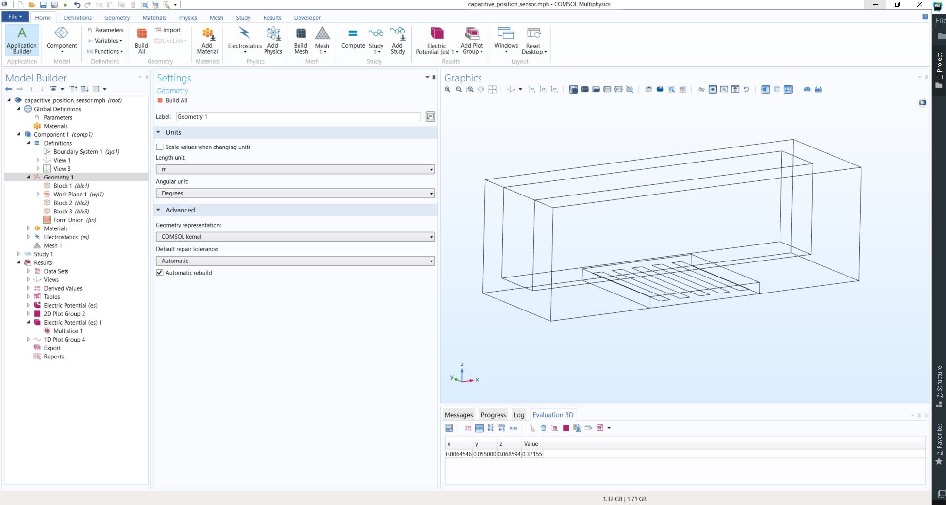
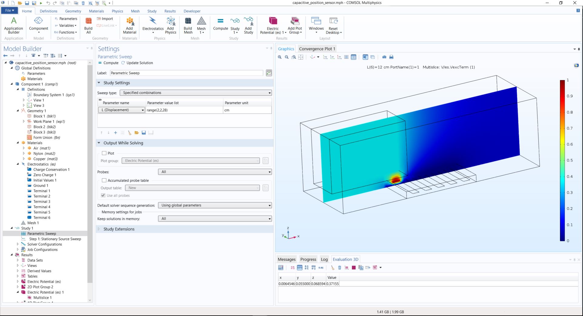
Tutorial #3: Capacitive Sensing

In this tutorial we are going to use the Electrostatic Module of COMSOL Multiphysics 5.3 to model an analog of capacitive position sensors. Specifically, the capacitance matrix of a five-terminals sensor is computed and related to the position of a metallic test object. The model utilizes the Stationary Source Sweep Study option to extract lumped matrices. Furthermore, we are going to see useful extra features of the Stationary Source Sweep Study, such as sweeping on a subset of the terminals are showcased. All the steps should give a nice overview of how to setup a COMSOL model to simulate interesting physics that can guide system design and implementation.
The classical workflow followed using an FEM-based simulation software is:

1) Making the Geometry

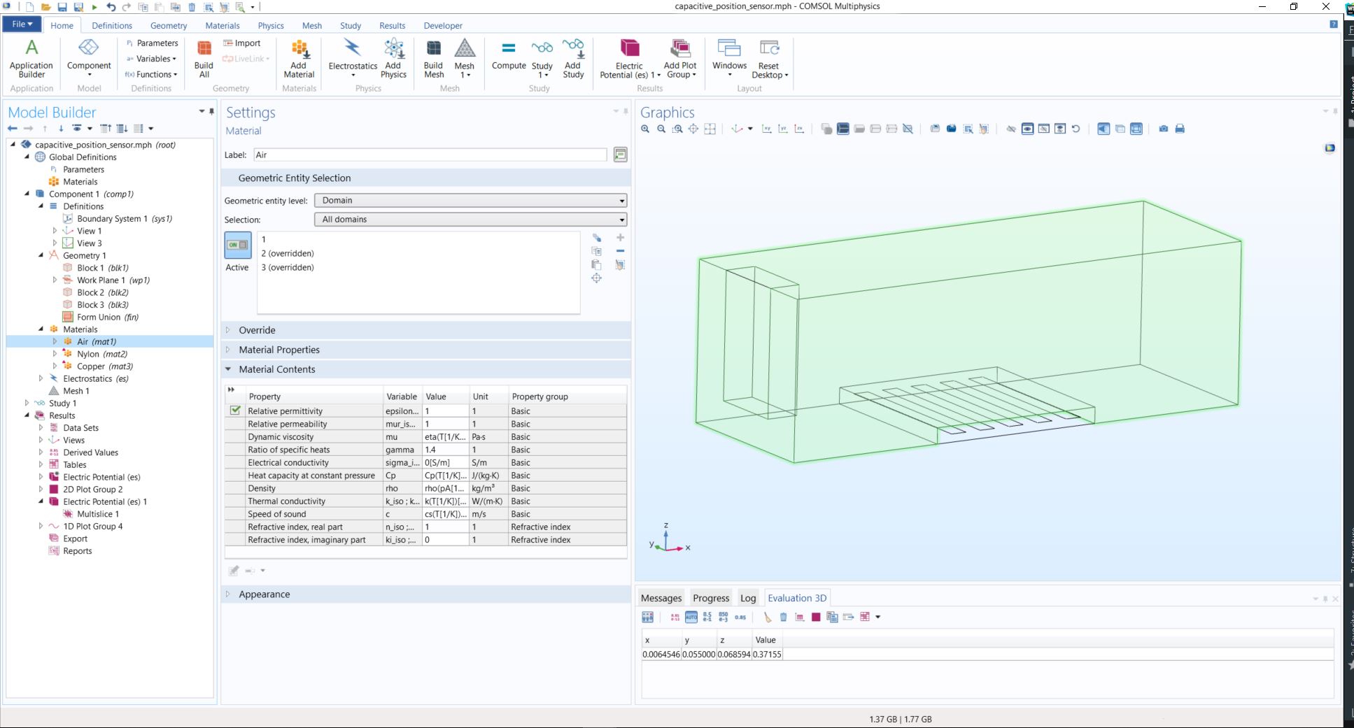
2) Assign Materials in domain or domains depending on your simulation scenario

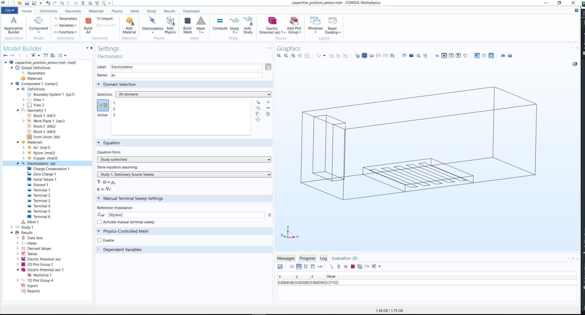
3) Setup the Equations and Boundary Conditions

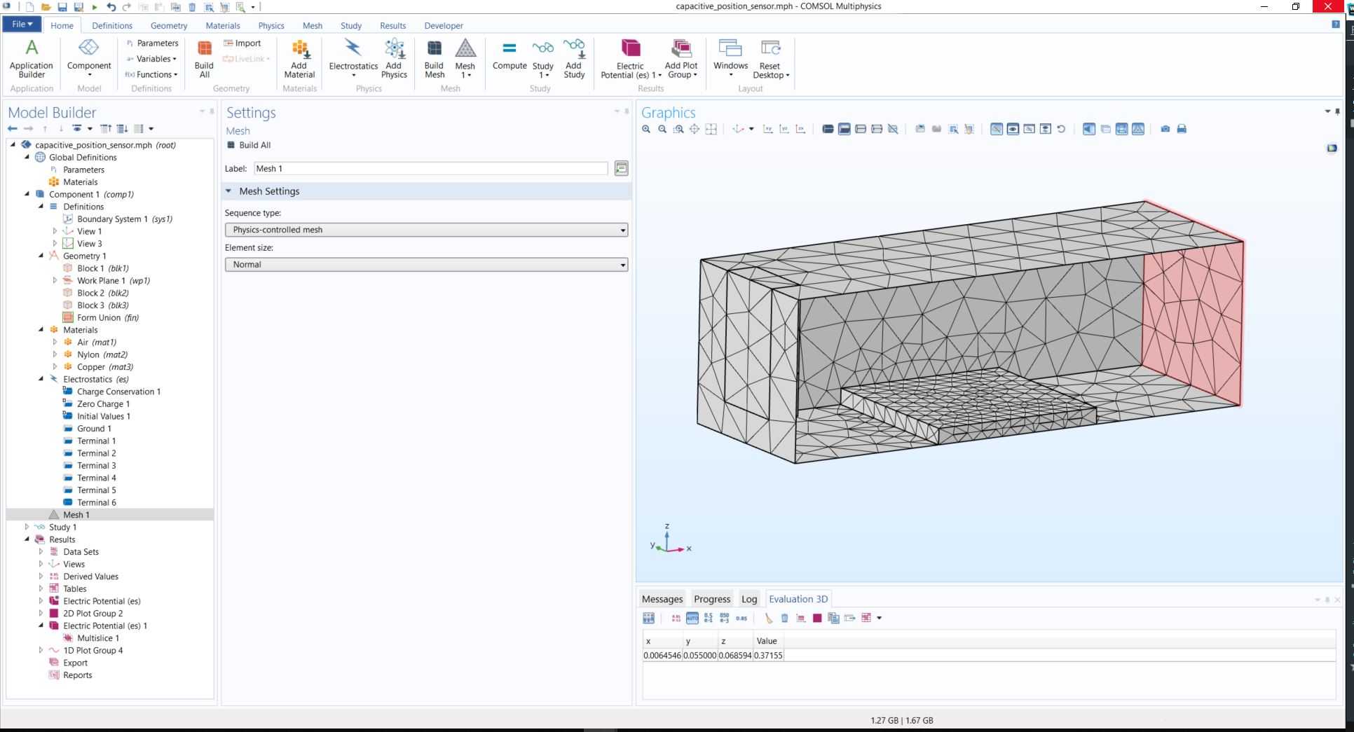
4) Mesh your geometry

5) Define type of Study and Compute

Now lets dig into the specific details of our model!

You can read more about capacitance calculation in Comsol HERE and more details about the specifics of the model HERE!